TileDB Global Database for GEDI Data#

Important

If you use the database for your publications, please acknowledge that the dataset has been processed using gediDB:

Besnard, S., Dombrowski, F., & Holcomb, A. gediDB [Computer software]. https://doi.org/10.5281/zenodo.13885229.

Overview#

The publicly available TileDB global database, managed by the Global Land Monitoring group at GFZ-Potsdam, stores all processed GEDI version 2 data with a robust and scalable architecture. All granules for the products L2A, L2B, L4A, and L4C have been ingested into the database. The data is stored in a Ceph object storage managed by the GFZ data center, with a current size of approximately 20TB. It enables efficient spatial, temporal, and attribute-based queries. This page provides an overview of the database setup, configuration, and access methods using the gediDB package.

Ceph Object Storage Configuration#

The TileDB global database utilizes a Ceph object storage backend to efficiently manage and distribute GEDI data. Below are the key characteristics of the Ceph bucket:

Bucket Name: dog-ext.gedidb.gedi-l2-l4-v002.0
Access Endpoint: https://s3.gfz-potsdam.de
Region: eu-central-1
Total Storage Used: ~13TB
Access Control: Public
Query Support: Optimized for spatial and temporal queries

For users accessing the database programmatically, interactions with the Ceph bucket are abstracted by the gediDB package, which retrieves data seamlessly from TileDB. Advanced users with direct access to the Ceph storage layer may utilize S3-compatible tools (such as aws s3api or rclone) to interact with the data.

Warning

The bucket dog.gedidb.gedi-l2-l4-v002 has been deprecated and is no longer maintained. Please update any existing scripts or configurations to use the new bucket dog-ext.gedidb.gedi-l2-l4-v002.0.

TileDB Database Configuration#

The database configuration defines key parameters for data storage, tiling, and query efficiency. A critical aspect of the database is the application of spatial consolidation, where fragments belonging to the same 10x10-degree spatial windows are consolidated together. This strategy significantly enhances query performance by reducing the number of fragments accessed during spatial queries.

Below is the structure of the configuration file used to build the TileDB database:

# database parameters
tiledb:
  storage_type: 's3'
  s3_bucket: "dog-ext.gedidb.gedi-l2-l4-v002.0"
  url: "https://s3.gfz-potsdam.de"
  overwrite: true
  temporal_batching: "annual"
  time_range:
    start_time: "2019-01-01"
    end_time: "2030-12-31"
  spatial_range:
    lat_min: -56.0
    lat_max: 56.0
    lon_min: -180.0
    lon_max: 180.0
  dimensions: ['latitude', 'longitude', 'time']
  consolidation_settings:
    fragment_size: 200_000_000_000   # 200 GB target fragment size
    memory_budget: "8589934592"      # 8 GB read buffer
    memory_budget_var: "4294967296"  # 4 GB for variable-length attributes
  cell_order: "hilbert"
  capacity: 200000
  latitude_tile: 6
  longitude_tile: 6
  flush_every: 200

The configuration file contains:

Storage Type: Specifies s3 for cloud-based storage.
Time Range: Defines the global temporal coverage.
Spatial Range: Sets the global bounding box for latitude and longitude.
S3 Settings: Configures connection and request parameters for S3.

Note

The current database architecture is somewhat experimental, and different approaches may be more suitable to improve the speed of spatial and temporal queries. Users are encouraged to provide feedback and suggestions for optimizing the tileDB database configuration.

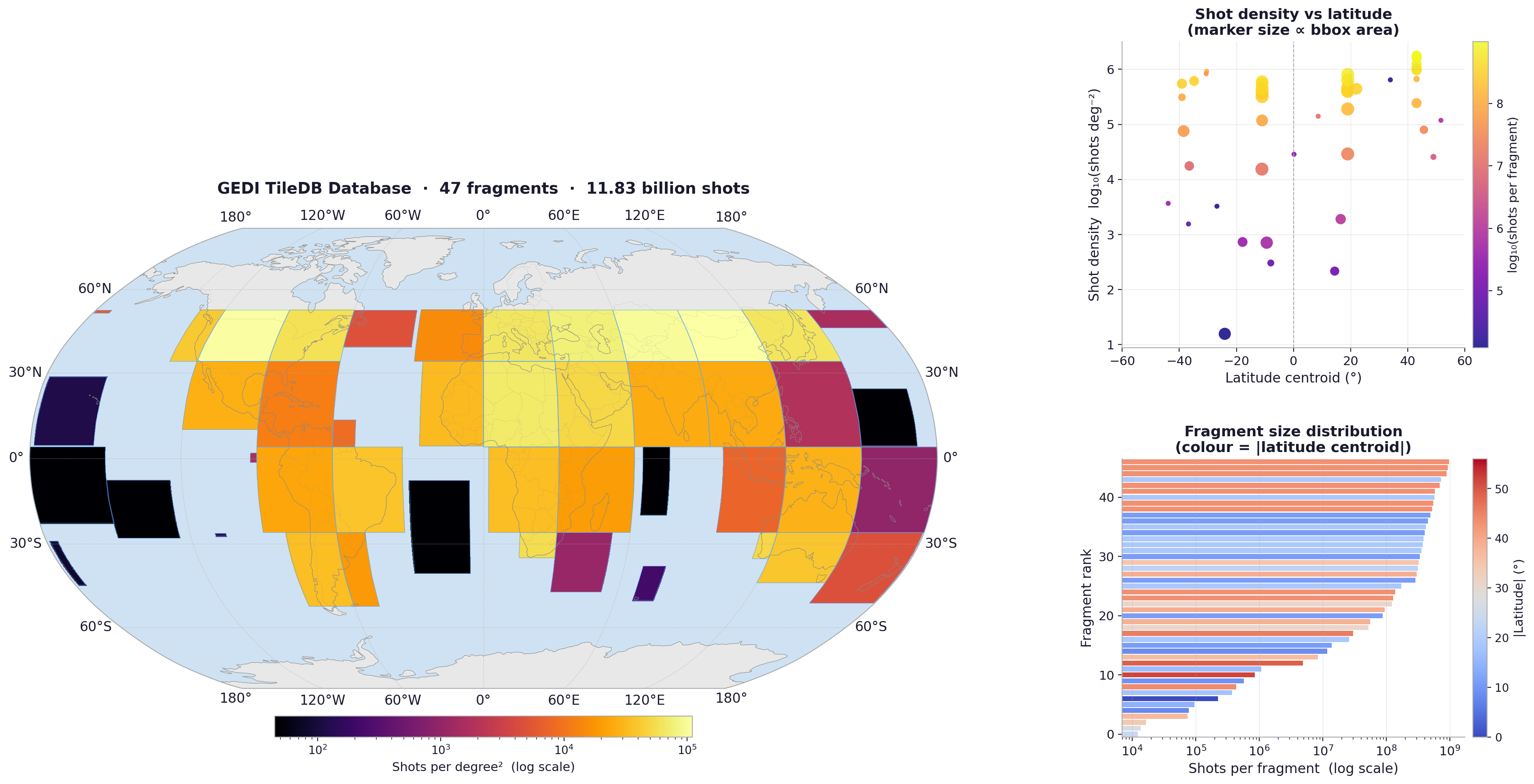
Data structure of the tileDB array — **Figure 2**: Internal storage structure of the GEDI TileDB database. The left panel shows the global distribution of TileDB fragments (blue outlines) overlaid on a log-scale shot density heatmap (shots per degree²). The top-right panel shows shot density as a function of latitude, reflecting the latitudinal gradient in GEDI orbital coverage. The bottom-right panel shows the fragment size distribution ranked by shot count, coloured by absolute latitude centroid.#

List of the available variables#

The database includes a wide range of variables, covering spatial coordinates, elevation data, vegetation metrics, biomass estimates, and quality flags across multiple GEDI products (L2A, L2B, L4A, L4C). Below is a table of available variables stored in the database:

Variable Descriptions#
Variable Name	Description	Units	Product
agbd	Aboveground biomass density	Mg/ha	L4A
agbd_a1	Aboveground biomass density - algorithm setting group 1	Mg/ha	L4A
agbd_a2	Aboveground biomass density - algorithm setting group 2	Mg/ha	L4A
agbd_a5	Aboveground biomass density - algorithm setting group 5	Mg/ha	L4A
agbd_pi_lower	Lower prediction interval for aboveground biomass density	Mg/ha	L4A
agbd_pi_upper	Upper prediction interval for aboveground biomass density	Mg/ha	L4A
agbd_se	Standard error of aboveground biomass density	Mg/ha	L4A
agbd_t	Model prediction in fit units	adimensional	L4A
agbd_t_se	Model prediction standard error in fit units	adimensional	L4A
algorithmrun_flag	The L2B algorithm run flag	adimensional	L2B
beam_name	Name of the beam	adimensional	L2A
beam_type	Type of beam used	adimensional	L2A
cover	Total canopy cover	Percent	L2B
cover_z	Cumulative canopy cover vertical profile [profile: 30 height bins, 0-145 m]	Percent	L2B
cp_height	Canopy profile relative height metrics at 1% interval [profile: 101 percentile points, 0-100]	Meters	L2B
cp_pavd	Canopy profile Plant Area Volume Density at 1% interval [profile: 101 percentile points, 0-100]	m²/m³	L2B
degrade_flag	Flag indicating degraded state of pointing and/or positioning information	adimensional	L2A
digital_elevation_model	TanDEM-X elevation at GEDI footprint location	Meters	L2A
digital_elevation_model_srtm	STRM elevation at GEDI footprint location	Meters	L2A
dz	Vertical step size of foliage profile	Meters	L2B
elev_highestreturn_a1	Elevation of the highest return detected using algorithm 1, relative to reference ellipsoid	Meters	L2A
elev_highestreturn_a2	Elevation of the highest return detected using algorithm 2, relative to reference ellipsoid	Meters	L2A
elev_lowestmode	Elevation of center of lowest mode relative to reference ellipsoid	Meters	L2A
energy_total	Total energy detected in the waveform	adimensional	L2A
fhd_normal	Foliage Height Diversity	adimensional	L2B
l2_quality_flag	Flag identifying the most useful L2 data for biomass predictions	adimensional	L4A
l2a_quality_flag	L2A quality flag	adimensional	L2B
l2b_quality_flag	L2B quality flag	adimensional	L2B
l4_quality_flag	Flag simplifying selection of most useful biomass predictions	adimensional	L4A
landsat_treecover	Tree cover in the year 2010, defined as canopy closure for all vegetation taller than 5 m in height as a percentage per output grid cell	Percent	L2A
landsat_water_persistence	Percent UMD GLAD Landsat observations with classified surface water	Percent	L2A
leaf_off_doy	GEDI 1 km EASE 2.0 grid leaf-off start day-of-year	adimensional	L2A
leaf_off_flag	GEDI 1 km EASE 2.0 grid flag	adimensional	L2A
leaf_on_cycle	Flag that indicates the vegetation growing cycle for leaf-on observations	adimensional	L2A
leaf_on_doy	GEDI 1 km EASE 2.0 grid leaf-on start day-of-year	adimensional	L2A
modis_nonvegetated	Percent non-vegetated from MODIS MOD44B V6 data	Percent	L2A
modis_nonvegetated_sd	Percent non-vegetated standard deviation from MODIS MOD44B V6 data	Percent	L2A
modis_treecover	Percent tree cover from MODIS MOD44B V6 data	Percent	L2A
modis_treecover_sd	Percent tree cover standard deviation from MODIS MOD44B V6 data	Percent	L2A
num_detectedmodes	Number of detected modes in rxwaveform	adimensional	L2A
omega	Foliage Clumping Index	adimensional	L2B
pai	Total Plant Area Index	m²/m²	L2B
pai_z	Plant Area Index profile [profile: 30 height bins, 0-145 m]	m²/m²	L2B
pavd_z	Plant Area Volume Density profile [profile: 30 height bins, 0-145 m]	m²/m³	L2B
pft_class	GEDI 1 km EASE 2.0 grid Plant Functional Type (PFT)	adimensional	L2A
pgap_theta	Total Gap Probability (theta)	adimensional	L2B
pgap_theta_error	Total Pgap (theta) error	adimensional	L2B
predict_stratum	Prediction stratum name for the 1 km cell	adimensional	L4A
predictor_limit_flag	Prediction stratum identifier (0=in bounds, 1=lower bound, 2=upper bound)	adimensional	L4A
quality_flag	Flag simplifying selection of most useful data	adimensional	L2A
region_class	GEDI 1 km EASE 2.0 grid world continental regions	adimensional	L2A
response_limit_flag	Prediction value outside bounds of training data (0=in bounds, 1=lower bound, 2=upper bound)	adimensional	L4A
rg	Integral of the ground component in the RX waveform	adimensional	L2B
rh	Relative height metrics at 1% interval [profile: 101 percentile points, 0-100]	Meters	L2A
rh100	Height above ground of the received waveform signal start	cm	L2B
rhog	Volumetric scattering coefficient (rho) of the ground	adimensional	L2B
rhog_error	Rho (ground) error	adimensional	L2B
rhov	Volumetric scattering coefficient (rho) of the canopy	adimensional	L2B
rhov_error	Rho (canopy) error	adimensional	L2B
rossg	Ross-G function	adimensional	L2B
rv	Integral of the vegetation component in the RX waveform	adimensional	L2B
rx_algrunflag	Flag indicating signal was detected and algorithm ran successfully	adimensional	L2A
rx_maxamp	Maximum amplitude of rxwaveform relative to mean noise level	adimensional	L2A
rx_range_highestreturn	Range to signal start	Meters	L2B
sd_corrected	Noise standard deviation, corrected for odd/even digitizer bin errors based on pre-launch calibrations	adimensional	L2A
selected_algorithm	Identifier of algorithm selected as identifying the lowest non-noise mode	adimensional	L2A
selected_l2a_algorithm	Selected L2A algorithm setting	adimensional	L2B
selected_rg_algorithm	Selected R (ground) algorithm	adimensional	L2B
sensitivity	Maxmimum canopy cover that can be penetrated	adimensional	L2A
sensitivity_a1	Geolocation sensitivity factor A1	adimensional	L2A
sensitivity_a2	Geolocation sensitivity factor A2	adimensional	L2A
shot_number	Unique identifier for each shot	adimensional	L4C
solar_azimuth	Solar azimuth angle at the time of the shot	Degrees	L2A
solar_elevation	Solar elevation angle at the time of the shot	Degrees	L2A
stale_return_flag	Flag indicating return signal above detection threshold was not detected	adimensional	L2B
surface_flag	Identifier of algorithm selected as identifying the lowest non-noise mode	adimensional	L2A
toploc	Sample number of highest detected return	adimensional	L2A
urban_proportion	The percentage proportion of land area within a focal area surrounding each shot that is urban land cover.	Percent	L2A
wsci	Waveform Structural Complexity Index	adimensional	L4C
wsci_pi_lower	Waveform Structural Complexity Index lower prediction interval	adimensional	L4C
wsci_pi_upper	Waveform Structural Complexity Index upper prediction interval	adimensional	L4C
wsci_quality_flag	Waveform Structural Complexity Index quality flag	adimensional	L4C
wsci_xy	Horizontal Structural Complexity	adimensional	L4C
wsci_xy_pi_lower	Horizontal Structural Complexity lower prediction interval	adimensional	L4C
wsci_xy_pi_upper	Horizontal Structural Complexity upper prediction interval	adimensional	L4C
wsci_z	Vertical Structural Complexity	adimensional	L4C
wsci_z_pi_lower	Vertical Structural Complexity lower prediction interval	adimensional	L4C
wsci_z_pi_upper	Vertical Structural Complexity upper prediction interval	adimensional	L4C
zcross	Sample number of center of lowest mode above noise level	Nanoseconds	L2A

Profile variables#

Several variables are stored as per-shot vertical profiles — each cell in the database holds an array of values rather than a single scalar. When queried via gedidb.GEDIProvider, full profiles are returned as a list per shot. Individual profile points can be fetched using the "variable:label" syntax (see Data Provider).

Profile variable details#
Variable	Product	Profile labels	Label meaning	Length
`rh`	L2A	0, 1, 2, …, 100	Percentile	101
`cp_height`	L2B	0, 1, 2, …, 100	Percentile	101
`cp_pavd`	L2B	0, 1, 2, …, 100	Percentile	101
`cover_z`	L2B	0, 5, 10, …, 145	Height above ground (m)	30
`pai_z`	L2B	0, 5, 10, …, 145	Height above ground (m)	30
`pavd_z`	L2B	0, 5, 10, …, 145	Height above ground (m)	30

Note

Percentile-profile variables (rh, cp_height, cp_pavd)

These variables store 101 values per shot, one per integer percentile of the canopy height or PAVD distribution (0 - 100). In the returned xarray.Dataset they appear as a 2-D variable with a named profile_points coordinate carrying the percentile integers:

ds = provider.get_data(variables=["rh"], ...)
ds.rh.sel(profile_points=98)   # 98th-percentile canopy height
ds.rh.sel(profile_points=50)   # median canopy height

Height-bin profile variables (cover_z, pai_z, pavd_z)

These variables store 30 values per shot at 5 m height steps from 0 to 145 m above ground. The profile_points coordinate carries the bin midpoints in metres:

ds = provider.get_data(variables=["cover_z"], ...)
ds.cover_z.sel(profile_points=50)    # cumulative cover at 50 m height
ds.cover_z.sel(profile_points=0)     # cover at ground level

Single-label selection (saves bandwidth — reads one column instead of all)

Use the "variable:label" syntax to fetch a single profile element at query time. The result is renamed {variable}_p{label}:

# Percentile: fetch only the 98th-percentile canopy height
df = provider.get_data(variables=["rh:98"], return_type="dataframe", ...)
# → column named 'rh_p98'

# Height bin: fetch cumulative cover at 50 m only
df = provider.get_data(variables=["cover_z:50"], return_type="dataframe", ...)
# → column named 'cover_z_p50'

# Mix profiles and scalars freely
df = provider.get_data(variables=["agbd", "rh:98", "cover_z:50"], ...)

See Data Provider for full details on the query syntax.

Accessing the database#

The gediDB Python package simplifies access to the TileDB global database. Below is an example workflow for querying data.

Example Code:

import geopandas as gpd
import gedidb as gdb

# Instantiate the GEDIProvider
provider = gdb.GEDIProvider(
    storage_type='s3',
    s3_bucket="dog-ext.gedidb.gedi-l2-l4-v002.0",
    url="https://s3.gfz-potsdam.de"
)

# Load region of interest (ROI)
region_of_interest = gpd.read_file('path/to/test.geojson')

# Define variables to query and quality filters
vars_selected = ["agbd", 'rh']

# Query data
gedi_data = provider.get_data(
    variables=vars_selected,
    query_type="bounding_box",
    geometry=region_of_interest,
    start_time="2018-01-01",
    end_time="2024-07-25",
    return_type='xarray'
)

Explanation:

GEDIProvider: Initializes the provider with S3 storage details.
Region of Interest: Defines the geographic area for the query using a GeoJSON file.
Variables: Specifies the variables to extract (e.g., agbd, rh).

Examples and use cases#

Here are some example use cases:

Retrieve Aboveground Biomass Density (AGBD) for a region:

gedi_data = provider.get_data(
    variables=["agbd"],
    query_type="bounding_box",
    geometry=region_of_interest,
    start_time="2018-01-01",
    end_time="2024-07-25",
    return_type='xarray')

Analyze Relative Heights (RH) with additional quality filters:

quality_filters = {"sensitivity": ">= 0.9 and <= 1.0", "beam_type": "== 'full'"}

gedi_data = provider.get_data(
    variables=["rh"],
    query_type="bounding_box",
    geometry=region_of_interest,
    start_time="2018-01-01",
    end_time="2024-07-25",
    return_type='xarray',
    **quality_filters)

Query performance#

Query time scales with the spatial extent of the bounding box. The benchmark was run on a Linux server with dual Intel® Xeon® E5-2643 v4 CPUs (12 cores, 24 threads) and 503 GB RAM, querying data stored on a Ceph object storage cluster (Quincy) comprising 18× DELL R7515 nodes, each equipped with 11-18× 18-20 TB data drives and 1× 1.6 TB NVMe for metadata.

The figure below shows wall-clock query time (and time per km²) as a function of bounding box area for 20 square bounding boxes of increasing size (0.5°-40° side length), all centred on central Europe (51°N, 10°E) and queried over a fixed one-year window (2020). Each box size was repeated three times and the median time is reported. A global archive query over the same period is included as a reference point.

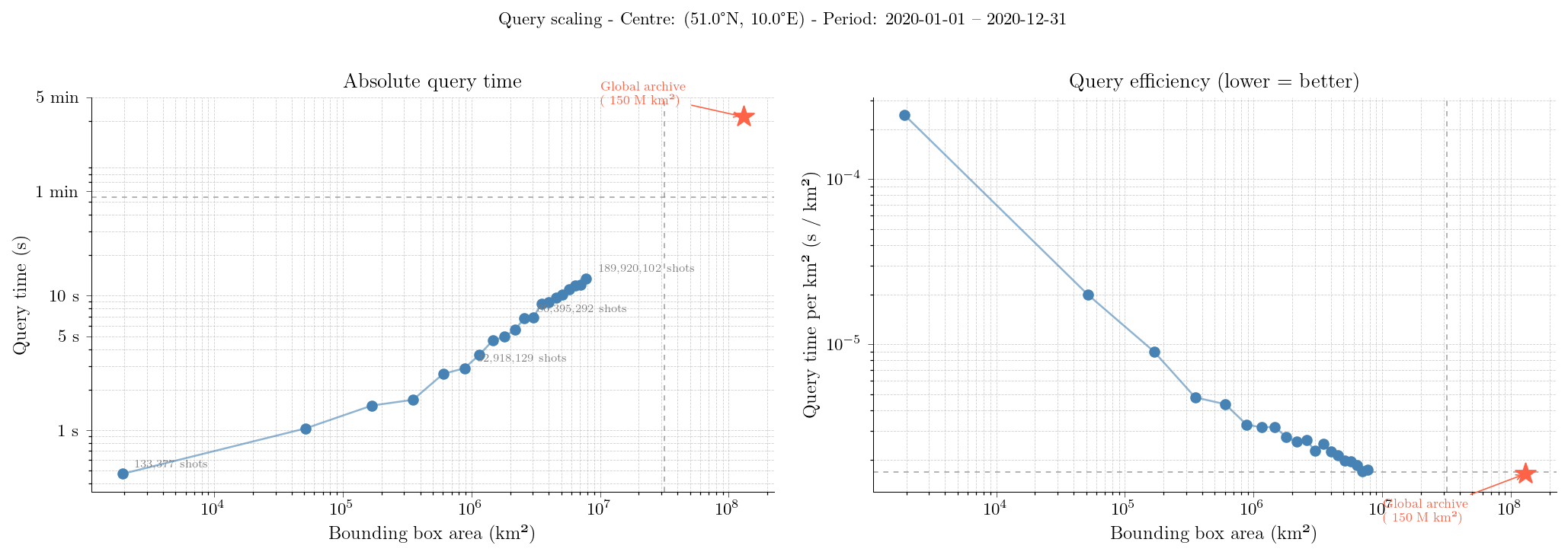
Query time vs bounding box area — **Figure 3**: Query scaling for the GEDI TileDB database. *Left*: absolute wall-clock query time (s) as a function of bounding box area (km²). *Right*: query time per km², a measure of query efficiency — lower values indicate more efficient use of the consolidated fragment structure for larger spatial extents.#